|
A few weeks back got a chance to attend Oracle’s Real World performance tuning class. This class was using Exadata hardware and Oracle 12c edition. A very interesting set of findings that I would like to present here:-
0 Comments
A typical Informatica MDM implementation uses Informatica ETL tool for processing data to the Landing tables, and may have one or more stages, depending on the architecture, for processing data from various in house or third party data providers; processing from Landing to Staging to Various target tables(cross reference, and associated tables), tokenization of these records and then match merge in the Informatica MDM space; and then generating feeds to various downstream data marts, data warehouses, OLTP systems, and third parties. In my experience a majority of this work happens with the Powercenter and MDM toolsets from Informatica. Though in this realm work can be and is done using Web Services, but for the purpose of this article, I shall ignore that use case. Once a system is in place, it needs to be monitored for ensuring ongoing data quality and performance. This tends to be a tedious task because not only are there multiple stages to the whole processing before, during and after MDM processing of the data, but also the performance metrics are stored in two different repositories. This article show what data is available in those repositories and how one could set some naming patterns as part of the standards while architecting such a system that would make it not only possible, but approach the whole effort in an efficient manner. So let us explore what both the repositories provide, starting with Informatica Powercenter repository:- Powercenter repository provides and can be leveraged to get a multitude of reports as shown here. For the purpose of this blog I shall be using the following tables:- a) opb_task_inst b) opb_task_run_inst The first table could be queried to get the various workflows/worklets/sessions that are available in the repository. I use the following query to get the information about the workflow and the other artifacts contained therein in a hierarchical fashion. WITH session_cfg_info AS (SELECT * FROM (SELECT connect_by_root workflow_id the_workflow_id , Sys_connect_by_path (task_id, ',') full_task_id, ti.*, Sys_connect_by_path (instance_name, '/') fully_qualified_name FROM (SELECT * FROM opb_task_inst ta WHERE task_type <> 62 AND version_number = (SELECT Max (version_number) FROM opb_task_inst ti2 WHERE ti2.instance_id = ta.instance_id)) ti WHERE connect_by_isleaf = 1 START WITH ti.workflow_id IN (SELECT task_id FROM opb_task WHERE task_type = 71) CONNECT BY PRIOR ti.task_id =ti.workflow_id) q WHERE q.task_type <> 70), workflow_cfg_info AS (SELECT subject_id, task_id the_workflow_id, task_name FROM (SELECT subject_id, task_id, task_name, Row_number () over ( PARTITION BY subject_id, task_id ORDER BY version_number DESC) trn FROM opb_task WHERE task_type = 71) q WHERE q.trn = 1) SELECT f.subj_name folder_name, w.the_workflow_id ||full_task_id full_task_id, '/' ||w.task_name ||s.fully_qualified_name task_name, s.instance_name, s.instance_id, s.task_id FROM session_cfg_info s join workflow_cfg_info w ON ( s.the_workflow_id = w.the_workflow_id ) join opb_subject f ON ( f.subj_id = w.subject_id ) We shall come to the use of this result set later. Next we gather the run time information about various jobs that ran using the following query as a starting point. SELECT workflow_id, rn, workflow_run_id, worklet_run_id, child_run_id, task_id, instance_id, instance_name, workflow_id || SYS_CONNECT_BY_PATH (task_id, ',') full_task_id, start_time, end_time, SYS_CONNECT_BY_PATH (instance_name, '/') fully_qualified_name, run_err_code,run_err_msg,run_status_code,task_type FROM (SELECT workflow_id, workflow_run_id, worklet_run_id, child_run_id, task_id,instance_id,instance_name,start_time,end_time, run_err_code, REPLACE (run_err_msg, CHR (10), ' ') run_err_msg, DECODE (run_status_code, 1, 'Succeeded', 2, 'Disabled', 3, 'Failed', 4, 'Stopped', 5, 'Aborted', 6, 'Running', 15, 'Terminated', 'Other' ) run_status_code, task_type, CASE WHEN child_run_id = 0 THEN -1 * (ROW_NUMBER () OVER (ORDER BY end_time, start_time) ) ELSE child_run_id END rn FROM opb_task_inst_run t WHERE task_type <> 62) q WHERE CONNECT_BY_ISLEAF = 1 CONNECT BY NOCYCLE PRIOR rn = worklet_run_id AND PRIOR workflow_run_id = workflow_run_id START WITH worklet_run_id = 0 Joining this information with the data from the opb_sess_task_log table, the opb_wflow_run tab and opb_subject table, one can derive the information to be able to join with the data from the workflow configuration data derived in the first query above. One has to be careful as the opb_sess_task_log will have higher cardinality than the workflow run query provide immediately above. If I am trying to monitor things at each and source qualifier or target level it, we could join it directly. However, if one is just trying to get a ball park idea of the volumes processed it might as well be aggregated, and that may provide good enough information for trending the performance numbers. For this exercise let us go with the latter:- SELECT workflow_run_id,instance_id, SUM (src_success_rows)src_success_rows, SUM (src_failed_rows) src_failed_rows, SUM (targ_success_rows) targ_success_rows, SUM (targ_failed_rows) targ_failed_rows, SUM (total_trans_errs) total_trans_errs FROM etl_prd_rep.opb_sess_task_log tl GROUP BY workflow_run_id, instance_id So having discussed the Powercenter repository queries, let us review the provided results. If your implementation is like any that I have seen at multiple organizations, you would find that the sessions running MDM job stored procedures are reporting either 1 or 0 rows processed, depending on how the stored procedure is being called. This just ends up giving the run timings. If you are lucky the implementation may even record error when the MDM job fails. But, the number of rows are not reported back. So to address this deficiency, let us move on the MDM repository schema. Here the queries are straight forward to obtain information about various jobs: SELECT jc.rowid_job job_run_id,jc.system_name data_system, jc.table_display_name subject_table_name,jc.object_desc job_desc, (SELECT job_status_desc FROM c_repos_job_status_type WHERE job_status_code = jc.run_status)run_status,status_message, (SELECT object_function_type_desc FROM c_repos_obj_function_type WHERE object_function_type_code = jc.object_function_type_code) job_type, jc.start_run_date start_date, jc.end_run_date end_date, jn.total_records, jn.inserted_records, jn.updated_records, jn.no_action_records, jn.matched_records, jn.updatedxref_records, jn.rejected_records, jn.tokenized_records FROM c_repos_table t JOIN c_repos_job_control jc ON (t.rowid_table = jc.rowid_table) LEFT OUTER JOIN (SELECT rowid_job, MAX (CASE WHEN metric_type_code = 1 THEN metric_value ELSE NULL END ) total_records, MAX (CASE WHEN metric_type_code = 2 THEN metric_value ELSE NULL END ) inserted_records, MAX (CASE WHEN metric_type_code = 3 THEN metric_value ELSE NULL END ) updated_records, MAX (CASE WHEN metric_type_code = 4 THEN metric_value ELSE NULL END ) no_action_records, MAX (CASE WHEN metric_type_code = 5 THEN metric_value ELSE NULL END ) matched_records FROM c_repos_job_metric jm GROUP BY rowid_job) jn ON (jc.rowid_job = jn.rowid_job) Again I chose to report the statistics in a row, but decided not to aggregate as that won’t always make sense to add these numbers. Also, I am showing only a few stats in the query, other metrics are available as well. Now, we come to the real challenge. The challenge lies in being able to combine the rows from the Informatica repository with those from the MDM repository. One could follow the approach whereby one could create characterize the data pulled from both the repositories with common attributes. Here we go back to the purpose of the very first query from this article. We could e.g. gather that data in a table where we could add extra attributes that would help us characterize those sessions/jobs. We would follow a similar approach in case of the MDM data. We would need to make sure that whenever we add new jobs on ETL/MDM side that we add those rows to these characterization tables. Using these characterization tables and knowing the fact that on a reasonably time synchronized platform the ETL jobs timing would be same or a little outside the MDM job timing, we could combine the rows exactly and get all the relevant stats from the MDM system. On a multi-domain MDM system the following attributes would be sufficient:- a. Domain (Customer/Product) b. Source System (Admin or others..) c. Operation (Landing, Staging, Loading, Auto Match & Merge, etc.) d. Table Name or MDM Target Object. For joining the ETL run information with the configuration don’t forget to use the fully qualified task id, as that takes care of the various shared objects use in multiple parent objects. While building one such system, I was able to use the various patterns in names to find these attributes. Since, I approached this problem after the fact of building the system in first place, this task was not trivial, but was made easy by a consistent use of naming conventions. If I was leading the build process I think this task can be further simplified, and can be more easily incorporated into the initial build itself. When doing a code review one looks to see if the best practices are followed. Some are about the readability and therefore maintainability of the code, but, then there are some which could point to application logic traps. While reviewing a SQL I found something in production code, leading me to believe it could/should have been caught more easily with a code review itself, though there is no excuse that it was not found with the data validation/qa step.
The pattern is as following:- Select grouping_attribute , max(descriptor_type_attribute), max(attribute_expiry_date) From table Group by grouping_attribute The data has to do with licensing of certain professionals, and the descriptor_type_attribute is the identifier given by the licensing board and will have any expiry date associated with it. This query would have been fine if both the attributes followed the same sorting strategy, but it was not the case. So one could end up picking up a license number(descriptor_type_attribute) with wrong expiry date. Not the intended outcome. Part of the fault in my humble opinion lies with giving a _no postfix to the descriptor_type_attribute in the data model. A better query could be written using the analytical functions in Oracle, e.g. Select grouping_attribute, descriptor_type_attribute, attribute_expiry_date from ( Select grouping_attribute, descriptor_type_attribute, attribute_expiry_date, Row_number() over(partition by grouping_attribute order by attribute_expiry_date desc) rn From table ) q Where q.rn=1 Continued from Columnar Databases I ...
So if a situation allows us to live with the limitations of the columnar databases, how good are columnar databases. To find out for myself I set up an experiment to compare a popular row based database (Oracle 11g) with compression turned on with a columnar database (Infobright) that relies on an open source database engine (MySQL). I also set the experiment to mainly explore the compression in storage, rather than any query performance as I did not have resource to set up that elaborate an experiment. For OLTP data structures(TCP-H(tm) Bench Mark) the Oracle compressed row data store used about 10 GB storage including some indexes, which are required for such databases. Infobright database on the other hand showed a 1.9GB. This is about 1/5th the storage required. This is a significant saving, when there are not a lot of indexes in row store, and if more indexes were added for performance reasons it would have shown even better comparison on storage requirements. For Star Schema Bench Mark database, the data extracts were of the range of 6.7 GB of raw ASCII data, when pulled from Infobright (it by default provides quoted strings, etc) vs. about 6 GB of raw ASCII data when pulled from Oracle tables, using custom pipe delimiter. When loaded into Infobright it compressed the data into a size of about 800MB, again using no indexes. When loaded into Oracle database with the same compression scheme as before the data used about 6.5GB. From these observations, we conclude that while Oracle provides compression, considering that we had 3 large indexes on the lineorder, and smaller indexes on smaller tables as well. However the columnar database (Inforbright) provided an order of magnitude compression compared to the raw text data and row store's (Oracle) equivalent database with basic compression. Due to lack of appropriate storage (exadata machine) I could not test the more aggressive compression scheme available from Oracle row store database. Query timings were better in case of Infobright database where the large fact table extraction to flat file took about 12 minutes and in case of Oracle the same took about 42 minutes. Thus highlighting the benefits of smaller storage, at the least, as the queries did not use any index for Oracle either as these queries gets all the data from the tables in the join. The star schema shows a higher compression ratio for the columnar database, even though, it uses mainly numeric type data types in the large fact table. References:- Abadi, D., Boncz, P., Harizopoulos, S. "Column-oriented Database Systems" in VLDB ’09, August 24-28, 009, Lyon, France. Abadi, D.J., Madden, S.R., and Ferreira, M. "Integrating compression and execution in column-oriented database systems" In Proc. SIGMOD, 2006. Hodak, W., Jernigan, Kevin, "Advanced Compression with Oracle Database 11g Release 2" An Oracle White Paper from Oracle corporation, September 2009 Oracle, "Oracle 11g SQL Reference Guide" from otn.oracle.com Oracle, "Oracle 11g Utilities Guide" from otn.oracle.com Inforbright.org, "Direct data load guide" available from inforbright.org With the need for processing more and more data and also the availability for more data captured electronically from various data collection points through commercial, non-profit, government or research communities. This phenomenon is termed as Big Data in industry parlance. To make sense out of
this data being gathered it requires large amount of processing power. This data may be available in granular form or as documents, and sometimes both may be co-related. Over the period of time we notice that the nature of the data gathered is getting changed. Traditionally most of the data was transactional in nature, requiring CRUD(create, update, delete) operations. Now a larger amount of data is being created that is usually not updated and may only be deleted when it is no longer needed, usually after a longer period of time than in the transactional sense. While OLTP database provided the ability to store the CRUD operations with ACID(atomic, consistent, isolated and durable) properties for handling more granular data, they were then enhanced to add storage of various types of documents(text, pictures, etc.) again with the OLTP type of transactions in mind. These databases typically use a normalized data model for storage. But the need for providing ACID guaranties, and to handle different type of data volumes for analytical needs, the data could no longer be contained in those models. Therefore the data warehouses were designed using same type of databases, but with different type of data models (typically dimensional, though not always). Data warehouses allowed separation of data from the OLTP systems, but still grew fairly large in volumes, and typically serve more read type operations than frequent updates or writes. While working with large volumes of data, I noticed that at times a large number of columns in a table have low cardinality, but the overall size of the table itself may be fairly large. This led me to believe that one could reduce the size of the data as stored on the disk if compression techniques are used. Since disk access is usually the slowest part of the access of a database a smaller footprint of data would presumably lead to faster retrieval of the data from the slower medium, however, there would be associated CPU cost that would be incurred in compressing the data. Since data warehouses carry the largest amounts of data there presumably would be tradeoff scenarios in using one or the other technique. Even though the normalization theory is about reducing the redundancy of duplicate data, and therefore providing most efficient storage, there has to be other techniques that could be combine with this to reduce the overall query timing. One of the recent technologies that focus on this aspect is the columnar storage based databases. [Abadi, Boncz, Harizopoulos, 2009] provide a brief introductory, tutorial to the columnar databases. They describe the columnar databases as "Column-stores, in a nutshell, store each database table column separately, with attribute values belonging to the same column stored contiguously, compressed, and densely packed, as opposed to traditional database systems that store entire records (rows) one after the other." They trace the history of the column stores back to 1970s, when the usage of transposed files were explored. In 1980s the benefits of decomposed storage mode(DSM) over row based storage were explored. Its only in 2000s that these data stores finally took off. Because of the affinity of the data values stored contiguously on disk pages for each of the columns the data lends to better compression schemes, that may be light weight in their CPU utilization but still provide heavy compression. However, these databases are challenged in their ability to provide updates and also in tuple construction required for use in applications which access data through ODBC/JDBC type interfaces. The tuple construction is required to present the data in row format used by these access applications. Continued at Columnar Databases II Since we could use the operators available from the SQL provided in my previous post from Informatica, it could be translated easily into an Informatica map. The attached diagram is self explanatory. The SQL override specifies a sort order by col1. To get a predictable output every time with same data in the table, it could be sorted on col1 & col2 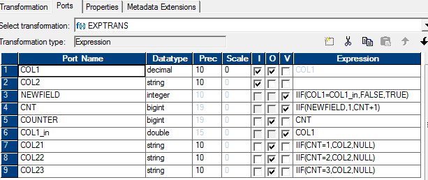 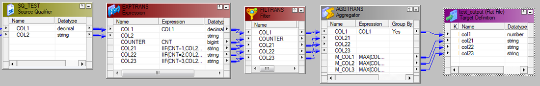 When I was interviewed the approach I took was on these lines:-
SELECT col1, MAX(CASE WHEN rn = 1 THEN col2 ELSE NULL END ) col21, MAX(CASE WHEN rn = 2 THEN col2 ELSE NULL END ) col22, MAX(CASE WHEN rn = 3 THEN col2 ELSE NULL END ) col23 FROM (SELECT col1,col2,row_number() over (partition BY col1 order by col2) rn FROM test ) GROUP BY col1 The results were same as from the previous post Interviews are always fun, but some make them even more interesting by asking questions about things that you never really got to handle in practice, but you generally know the context. They test your ability to think on your feet, if not exactly, your knowledge... One such question I got was, how you would pivot a table with columns (col1 number & col2 varchar2) with data such that there are maximum 3 rows per a distinct value in col1, and the desired output is col1, col21, col22, col23. Whereas I have worked with pivoting data that could be aggregated, text data type for column col2 makes it more interesting. Here is one possible solution using SQL in Oracle database, create table test( col1 number(10), col2 varchar2(10)); insert into test values(1,'a'); ... insert into test values(3,'c'); commit; with t as( select col1, col2, row_number() over (partition by col1 order by col2) rn from test ) select a.col1, a.col2 col21, b.col2 col22, c.col2 col23 from ( select col1, col2 from t where rn = 1) a left outer join ( select col1, col2 from t where rn = 2) b on ( a.col1 = b.col1) left outer join ( select col1, col2 from t where rn = 3) c on ( b.col1 = c.col1) 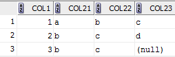 There won't be many times, but sometimes you may need to drop/recreate indexes on the CMX_ORS tables to typically re-import data. The following code PL/SQL code snippets shows how to do it.
Dropping Indexes CREATE OR REPLACE PROCEDURE drop_ors_indexes( in_table_name IN VARCHAR2) AS ddlText VARCHAR2(1000); CURSOR constraint_ IS SELECT t.table_name, replace(trim(k.rowid_key_constraint,'.','_')) rowid_key_constraint FROM C_REPOS_TABLE t, C_REPOS_KEY_CONSTRAINT k ON ( t.rowid_table = k.rowid_table AND t.table_name = in_table_name) WHERE EXISTS ( SELECT 1 FROM USER_INDEXES u WHERE u.INDEX_NAME = replace(trim(k.rowid_key_constraint,'.','_')); BEGIN FOR rec IN constraint_ LOOP ddlText := 'DROP INDEX '||rec.rowid_key_constraint; execute immediate ddlText; END LOOP; END drop_ors_indexes; / Re-creating indexes CREATE OR REPLACE PROCEDURE create_ors_indexes(in_table_name IN VARCHAR2) AS Left as an exercise for the reader to create based on drop indexes. You would need to use C_REPOS_KEY_CONSTRAINT_COL to use the columns for the index. Tablespace name is also available from the C_REPOS_TABLE. BEGIN END create_ors_indexes; / |
About Sarbjit ParmarA practitioner with technical and business knowledge in areas of Data Management( Online transaction processing, data modeling(relational, hierarchical, dimensional, etc.), S/M/L/XL/XXL & XML data, application design, batch processing, analytics(reporting + some statistical analysis), MBA+DBA), Project Management / Product/Software Development Life Cycle Management. Archives
March 2018
Categories
All
|
 RSS Feed